 (x,t) = (
 1(x,t),...n(x,t)).
EDV-Zentrum der Karl-Franzens-Universität Graz, Universitätsstr. 27, A-8010 Graz
Institut f. Mathematik, Karl-Franzens-Universität Graz, Heinrichstr. 36, A-8010 Graz
Powerful software packages offer new possibilities for the interactive visualization of quantum mechanical wave functions describing particles with spin in three dimensions. We discuss several visualization methods in view of their ability to extract physically interesting information from the wave function. We describe the practical realization of these techniques using the modular software package AVS. In AVS, the user combines program modules into networks which perform the visualization task. This process is described in detail and applied to some interesting examples from quantum mechanics.
The visualization of natural phenomena is a rapidly growing field of increasing importance in all parts of science [1]. The graphical representation of scientific data might uncover hidden patterns or draw the attention to otherwise unnoticed details and thus might help to decide about the future direction of research. Visualization helps the teacher to explain interesting phenomena, increases the students familiarity with abstract concepts, and might even attract the attention of a wider audience to a particular field of science, as it happened, for example, with chaos and fractals.
The exploration and application of visualization techniques in quantum mechanics has a long tradition [2] and is particularly rewarding for it bears the fascination of showing objects that cannot be seen by any other means. The typical objects of a quantum mechanical theory are mathematically idealized concepts from which physical properties can only be derived by the application of certain interpretation rules. A picture of the wave function of an electron, would not show the particle as it "really" is. Instead, the wave function describes probabilities for finding certain values for physical observables like position, momentum, or spin during repeated measurements on identical systems (at least according to the most widely accepted interpretation). The main technical difficulty one has to face when trying to make this information visible is that usually very high dimensional data are given at each point of space and time. Hence in general it is not possible to visualize simultaneously all the information contained in the wave function. One has to concentrate on particular aspects, and to apply special techniques in order to extract the most interesting physical information in a form that can be visualized. This, of course, is a first step necessary for any visualization task in science. The second step is the concrete realization.
Until recently, the predominant methods of visualizing quantum mechanical processes have been black and white plots of simple wave functions in one and two dimensions. The great progress due to better computer hardware and the advent of new program packages has provided us with new techniques for a graphical representation of large amounts of complex data. This justifies a systematic exploration of the new possibilities and their impact on presentation, teaching and research. With the help of modern visualization packages there is a hope to display quantum mechanical processes in three dimensional space in a quick and useful way, without discarding too much of the physical information, and without the need for writing own program codes. In this article we are going to illustrate the possibilities offered in particular by the software package AVS ("Application Visualization System" licensed by Advanced Visual Systems Inc.) for the interactive exploration of high dimensional data. AVS has a steep learning curve and the information in the following sections should help the reader to get started with own projects. In particular, the interactive manipulation of three dimensional objects is one of the striking advantages of the software.
In Section 2 we propose some physically meaningful methods to extract information from high dimensional wave functions that is suitable for a graphical representation. In this section we explain the philosophy behind the visualizations shown in this article. In Section 3 we provide some background information on AVS and its usage. The basic method of using AVS consists in designing suitable networks of program modules in order to serve a particular visualization task. We describe some AVS networks which are particularly useful for the visualization of high dimensional data like wave functions, also their use is not restricted to quantum mechanics. In Section 4 we describe our sample wave functions and explain how the data have been prepared for input to AVS. In Section 5 we discuss the application of the AVS networks to the visualization of these wave functions. Our sample networks can be implemented quickly and used interactivly and in real time for the graphical exploration of wave functions. In Section 6 we discuss the obtained results.
We consider high dimensional "spinor" wave functions of the type
(x,t) = (1(x,t),...n(x,t)).
The components i represent an internal degree of freedom at each point of space time (for example, the spin angular momentum) and are usually complex-valued functions. For nonrelativistic electrons, we need n = 2, in 3 the relativistic case even n = 4 components. This leaves us with the problem of displaying four (resp. eight) real data values at each point of the four-dimensional space-time.
In principle, all information is contained in the real- and imaginary parts Rei, Imi of the components of the wave function . Hence one could do a
series of separate plots of the real- and the imaginary parts, each of which are
ordinary functions. But the splitting into real and imaginary part in fact has
no physical meaning, since the wave function can always be multiplied with
an overall phase factor exp(i ) without changing its physical interpretation. This would change completely the appearance of the plots. A better and physically more interesting way is to plot the absolute value of the wave function, or the square of the absolute value,
at each point (x,t). The square of the absolute value has a direct physical interpretation in terms of the position probability. Several methods are available for visualizing a real-valued function in three dimensions, e.g., isosurfaces, slice planes, etc.
If we discuss only the position probability density of a wave function, important physical information is missed. This is the information on the dynamical state of the particle as well as the information on its internal degree of freedom, the spin.
In case of two-component spinors (x) (particles with spin-1/2 in three dimensions) we will proceed as follows. We consider the following set of functions:
(for i = 0,1,2,3). Here  i, i = 1,2,3, are the Hermitian 2x2 Pauli matrices, 0 is the 2 x 2 identity matrix.
  0(x) is just the position probability density, while the three components i(x), i = 1,2,3, form the spin vector field which describes a local density of the spin expectation value.
A visualization of the three dimensional spin vector field can be done by attaching arrows to selected grid points or by flux lines (these are curves 4 for which the tangent vector at each point is determined by the vector field at that point). It is sometimes illustrative to include an isosurface for the function 0(x) in the same plot.
The functions i(x), i = 0,1,2,3, in turn determine (x) only up to a
phase factor. The replacement (x)  exp(i
exp(i (x)) (x) would change neither the
position probability nor the spin vector field. This phase factor is nevertheless
important, because it contains the information about the momentum and
velocity distribution in the wavepacket - at least if we assume that the gauge
has been fixed. (For example, in the force free case one would assume the
electric and magnetic potentials to be zero. In this case the complex phase is
unique up to a constant phase factor exp(i) which does not depend on the position or on time).
(x)) (x) would change neither the
position probability nor the spin vector field. This phase factor is nevertheless
important, because it contains the information about the momentum and
velocity distribution in the wavepacket - at least if we assume that the gauge
has been fixed. (For example, in the force free case one would assume the
electric and magnetic potentials to be zero. In this case the complex phase is
unique up to a constant phase factor exp(i) which does not depend on the position or on time).
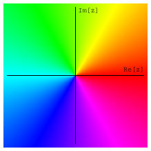
Fig.1: The color circle according to the RGB model is mapped to the complex plane in order to define a color code for the phase of a complex number.
In order to represent the complex phase of a wave function one can use an appropriate color code. The complex phase will be associated to a color by mapping the standard color circle of the RGB color model to the complex unit-circle in a one-to-one fashion as in Fig.1.
The plot of a wave function colored according to its phase provides simultaneous information on the position and momentum of the particle. Hence the distribution of colors in the wave packet gives some information about its future time evolution. In three dimensions the color information for the complex phase can be displayed by coloring isosurfaces of the absolute value or the position probability density.
In the following, we show how to implement these visualization methods - in particular the coloring of isosurfaces, plots of vector fields, etc. - for the program AVS and apply these methods to some interesting wave functions in three dimensions.
The Application Visualization System (AVS) is a product of Advanced Visual Systems Inc. The initial focus of AVS was to help the time-to-insight for research scientists by viewing the results of their simulations and experiments using interactive 2D images and 3D graphics. With AVS the scientist can analyze, manipulate and display large volumes of complex and multi-dimensional numerical data by using a visual programming environment. The independent computing elements which perform specific functions or sets of functions are represented by modules. With over 230 modules, AVS provides a very broad range of techniques for visualizing information. The module library runs the gamut of visualization, imaging and graphic functions and is fully customizable to meet a user's specific needs. The program is used in a variety of disciplines including engineering analysis, medical imaging, remote sensing, environmental studies, education and research [3].
AVS currently operates on all major UNIX and VMS workstations with the X- Windows system and supports the full range of graphics hardware available on these workstations. Within this year there will be an upgrade which is announced to introduce essentially new features (AVS/Express - the Visualization Edition) based on a different architecture, but built to accomplish the same goals. This upgrade includes support for both, MS- Windows and UNIX. AVS requires a minimum of 16 megabytes of physical memory. 32 or 64 megabytes of main memory are recommended. The minimum swap space should be two times either the available physical memory or 64 megabytes, whichever is greater. Moreover, the software occupies approximately 65 megabytes of disk storage. AVS uses two mechanisms for rendering geometric objects and scenes: The hardware renderer uses the native graphics hardware and the PHIGS graphics library. The software renderer implements a set of graphics primitives displaying the resulting image in a Window under the X- Window system.
A key component of the system architecture is the Data and Execution Model visualized in Fig.2.
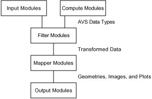
Fig.2: The Data and Execution Model schematically represents the data flow in an AVS network.
The diagram shows the visualization process, which begins with reading the input data and ends with output either to screen images or to a video/hard- copy output device. Each module can be considered a separate process dealing with the data. The network provides a data processing pipeline within which the output of one module is the input to the next one. The connection 7 between the modules controls the flow of data. This queue is ordered by the position within the network and by the time at which module parameters are changed.
AVS consists of the following subsystems:
* Network Editor: The Visual Programming Environment (Network Editor) allows the user to construct applications by picking the desired modules from the module libraries and connecting them interactively into a network which is visualized as a graph. The network defines an application which can be saved, reused and modified.
* Geometry Viewer: This subsystem adapts geometrical objects using the 3D rendering techniques isosurfaces, orthogonal and arbitrary slicers, streamlines, hedgehogs, particle advection, and the volume rendering techniques ray casting and 3D texture mapping.
* Image Viewer: It is an interactive tool for displaying, manipulating, and processing images.
* Graph Viewer: The Graph Viewer includes 2D plotting capabilities for generating x-y plots and contour plots.
AVS also supports some techniques for producing real-time animations. In addition there is the posibilty to extend the range and depth of the software by adding userdefined modules or by importing public domain modules.
Our sample wave functions describe stationary states of simple physical systems. As a first example we consider a highly exited state of the hydrogen atom. The wave function is given in analytic form, e.g., in [4]. We neglect the spin and consider a state with principal quantum number N = 10 and orbital angular momentum l = 5. The magnetic quantum number is m = 3 (third component of the orbital angular momentum vector). We also consider another state which is a superposition (with equal coefficients) of the states with m = 3 and m = -3. The wave function describing this superposition is particularly simple, because it is real-valued. Mathematically, it is equal to the real part of the wave function with m = 3.
The second example shows a zero energy state in a special three dimensional magnetic field, which was first described in [5], see also [6]. Since the possibility of zero energy bound states in a purely magnetic field in three dimensions depends on the spin of the particle, the most interesting information contained in the wave function (apart from the position probability density, which in this case is spherically symmetric) is the distribution of spin vectors.
The wave functions of the hydrogen atom and the zero energy state in a magnetic field can be expressed in terms of special functions and thus the numerical data for the AVS input are easy to obtain. For both examples we used Mathematica to calculate the wave functions, i(x), and the phase function (x) as described in Section 2. The values of these functions were then determined numerically on a regular three dimensional grid of points in cartesian coordinates and written to a file in ascii form. The data have, for example, the form
0.02672 0.02936 0.03194 0.03433 0.03639 ...
(Of course, one could also write the data as "byte" in order to save disk space). The output for each component of the multi-dimensional data is written to a separate file. These files then serve as input data files for AVS. The wave function of the hydrogen atom is sampled on a regular grid within a 50x50x50 cube (an edge roughly corresponds to 2.6*10-8 meters in international units). We are going to display the absolute value, the phase and the real part of the wave function. For example, the data file for the real part consists of 125000 numbers, separated by blanks. The data of the zero energy state in the magnetic field is calculated on a grid of 25x25x25 points. Here it is sufficient to calculate i, i = 0,1,2,3, because the phase is constant and may assumed to be zero.
We finally note that there are Mathematica/AVS modules available from MathSource [7] which allow a communication between Mathematica and AVS on a higher level.
We will discuss the process of the visualization in several steps. The starting point is to convert the data into an AVS-readable form. The scalar data (like absolute values of wave functions or real-valued wave functions) are visualized by slices and isosurfaces. In the case of high-dimensional data with vector components we use the techniques of streamlines and arrows to make vector fields visible. Finally we discuss the usability of animations
In order to read the data with the AVS module read field, it is necessary to write an AVS field file, which contains a simple description of the data in about 10 to 15 lines. The AVS field file format appears to become a kind of standard for multi-dimensional data [8]. Here we will give an example for such a field file in the case of the absolute value of the hydrogen wave function:
# AVS field file
ndim = 3
dim1 = 50
dim2 = 50
dim3 = 50
nspace = 3
veclen = 1
data = float
field = uniform
variable 1 H002abs.out filetype=ascii skip=0 offset=0 stride=1
The first five characters in the description file must be # AVS or read field will not recognize the file as valid. ndim is the number of computational dimensions in the field. nspace is the dimensionality of the physical space that corresponds to the computational space. veclen is the number of data values for each field element. In the case of multi-dimensional data veclen > 1. The data type can be byte, 2 bytes, integer, float and double. Since the data are calculated at regular distances, the field can take its mapping into the physical space from the organization of the computational array of field elements. variable specifies where to find the data, its type, and how to read them.
The simplest network (Fig.3) for reading this data and visualizing them in 2D would consist of the following steps:
* reading the data
* cutting the three dimensional data to produce 2D slices
* displaying them as an image.
Moreover the result can be colored by using a colormap. If problems occur during the data input one can use the module print field to check the dataset.
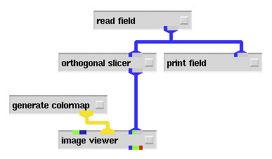
Fig.3:
Simple network for displaying 2D slices through a 3D dataset
In this way it is possible to display the different scalar components of the wave function such as the real and imaginary part, or the absolute value and the phase. They can be colored using an appropriate colormap. By changing the parameters of the module orthogonal slicer it is possible to "walk through" the dataset in x, y, and z direction. An even more interesting visualization technique is to transform the 2D scalar field to a surface in 3D space and to display more than one plane. Within AVS this is easily accomplished by inserting the module field to mesh between the modules orthogonal slicer and image viewer and by substituting the image viewer with the geometry viewer. The field to mesh module maps each element of the field to a mesh point. The 11 height of the mesh is proportional to the scalar value of the field. Another possibility is to replace the module orthogonal slicer by the arbitray slicer. The output data of this module form a geometric object which can be read directly by the geometry viewer. Fig.4. shows one slice through the absolut value of the wave function, and one slice through the phase data.
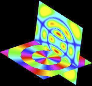
Fig.4:
Orthogonal slices through the wave function of the hydrogen atom with quantum numbers N = 10, l = 5, m = 3. The vertical plane shows the absolute value colored according to a built-in colormap in order to distinguish the values of the data. The horizontal plane displays the phase of the wave function with a colormap according to Fig.1.
The module isosurface allows for visualizion of the 3D structure of the data. It produces a geometric object that represents an isosurface of the data. An isosurface is a 3D generalization of a 2D contour line. It connects all field elements that have the same parameter-controlled data value. Fig.5 displays 12 a network using this technique.
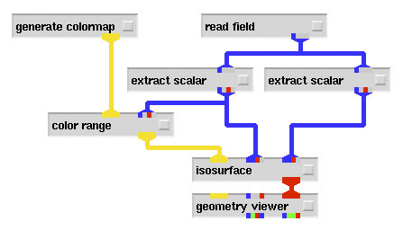
Fig.5:
A network for displaying a color-coded isosurface.
In this case the read field module inputs a field file with multi-dimensional data. Thus it is possible to read the different scalar components of the wave function (absolute value, phase, real part and imaginary part) using only one read field module. Subsequently with the extract scalar module one can extract the desired component. In the above network (Fig.5) the right extract scalar module sends the data of the absolute value of the wave function to the isosurface module in order to generate an isosurface, whereas the left extract scalar module sends the phase data to the isosurface module in order to color the isosurface. The color at each point of the surface indicates the value of the phase at this point. To produce a colored isosurface one must also specify a colormap. The low value and high value parameters of the generate colormap module have to correspond to the minimum and maximum data values of the phase data. The color range module scales the colormap to the range of the phase data. The resulting image an isosurface of the absolute value, the phase is color encoded according to Fig.1. Because the calculation of an isosurface is time consuming, it is advisable to include a downsize module in the network to reduce the size of data. Fig.6 demonstrates the result of this network.
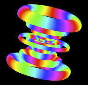
Fig.6:
The wave function of a highly excited hydrogen bound state with quantum numbers N = 10, l = 5, m = 3. The picture shows an isosurface of the absolute value of the wave function. The colors encode the phase according to the color circle convention in Fig.1. The diameter of this structure is about 3 * 10-8 meters.
The colordefects, which can be observed in the light-blue region of the isosurface, stem from an inappropriate behaviour of the interpolating algorithm in areas containing phase discontinuities.
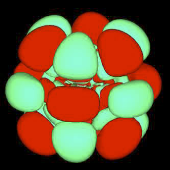
Fig.7:
Combination of two isosurfaces for a real-valued wave function of the hydrogen atom with quantum numbers N = 10, l = 5. The wave function describes a superposition of states with magnetic quantum numbers m = 3 and -3. The picture shows the positive and negative regions of the wave function. The red surface is an isosurface at some positive value, the green surface at the corresponding negative value of the real-valued wave function.
As described above, the data of the zero energy state in a magnetic field consists of both scalar data (probability density) and vector data (spin data). For visualizing these multi-dimensional data we use the UCD (unstructured cell data) data type which is provided within the AVS system. The data structure consists of an irregular coordinate structure made up of cells. The 15 data are structured as a set of components which can be either scalar or vector. The UCD data type is used as input for many useful AVS modules. The field to UCD conversion is performed by the module field to ucd.
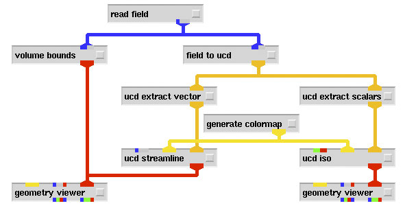
Fig.8:
A network for displaying the vector components of the wave function.
In a first step we want to visualize the spin structure of the zero energy state by streamlines and the probability density as an isosurface. As it is shown in Fig.8 we start with a read field module reading the four datafiles of the components i. In a next step the data are converted in UCD. From the UCD structure we can extract the scalar component for the probability density (ucd extract scalars) and the three vector components for the spin expectation values (ucd extract vector). An appropiate colormap is used to colorize the high values with red, the low ones with blue. The ucd streamline module generates colored streamlines based on the vector node data in the UCD structure by application of an euler integration method, or a 2nd order or 3rd order Runge-Kutta method.The streamlines are generated at selected sample points (e.g. in a plane). For every time step, the ucd streamline module moves each sample point through space, resulting in a set of stream lines which resemble the paths of massless particles moving under the influence of the vector force field. The sample probe places are parameter controlled, and they can be moved through the cube. The volume bounds module generates a bounding box for the data. In Fig.9 the plane of the sample probes is positioned in the middle of the sample cube and invisible, in Fig.10 the displayed 16 sample plane is translated along the z axis and rotated. The result of the calculation of the isosurface is not displayed in the same output window because the absolute value of the wave function is just spherically symmetric and therefore not very interesting.
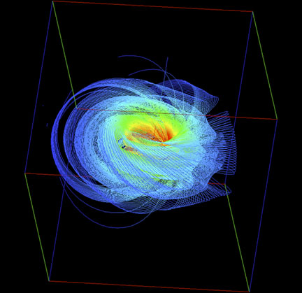
Fig.9:
A spin structure of the zero energy state in a magnetic field visualized by streamlines. The plane of the sample probes is positioned in the middle of the cube.
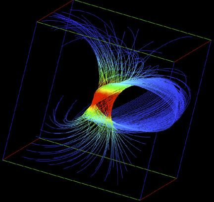
Fig.10:
As Fig.9, but this time the sample plane has been moved.
Another possibility of visualizing vector data is the use of arrows indicating the flow of the vector field. Replacing the ucd streamlines module by ucd hog show UCD node vector values as arrows in 3D space. ucd hog takes in a UCD structure whose nodes contain 3D vectors and displays these vectors as small line segments with a particular length, direction and color. As in the case of the streamlines the arrows are calculated starting from sample points along the sample line, circle, plane, or space. ucd hog either displays the arrows with white line segments of different length significating the magnitude of the vector or it associates a color with each line segment vector based on the magnitude of the vector. Fig.11 shows the same data as Fig.9, starting from the same sample plane, but with arrows instead of streamlines.
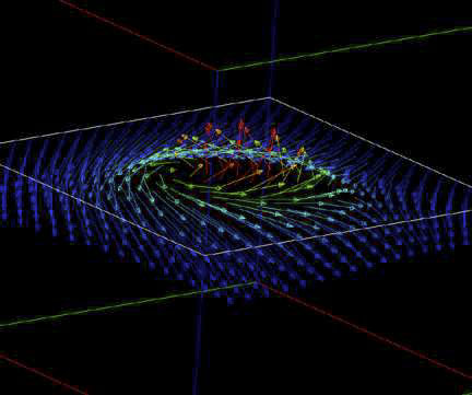
Fig.11: Spin structure of the zero energy state in a magnetic field visualized by arrows.
In the visualization of complex multi-dimensional data it is useful to build animations for displaying more information in a clearer way. In the case of the previously discussed networks it is meaningful to show the movement of the sample plane through the whole data. In this way it is possible to follow the direction and curvature of the streamlines, or to show different starting planes for the arrows indicating direction and size of the vector field. AVS offers possibilites to produce animations. But another idea is to use the public domain module create mpeg to build movies in the MPEG format. This requires less disk space and a simpler hardware for displaying the movie. The create mpeg module has to be connected with the output port of the geometry viewer. As a result every change of the displayed object in the geometry viewer window is sent to the create mpeg module. Because of the way MPEG movies are encoded by "MPEG", a lot of temporary disk space is 19 needed. After generating the movie all temporary files will be deleted. The execution time depends on the number of frames and their size. One can display the resulting movie at different computers, furthermore the movies can be included in the WWW [9].
The visualization of wave functions in 3D is a great tool for getting a quick overview of the qualitative features. In a first and simple step we visualize 2D slices of the three dimensional wave function of the hydrogen atom. In Fig.4 the absolute value of the wave function is displayed in the vertical plane. The red regions are the regions of the highest absolute value, whereas lower values are colored in green and blue. The horizontal slice visualizes the phase of the wave function with a color map according to Fig.1.
Visualizing the wavefunction as a real geometric object results in a more significant figure. For example, a look at Fig.6 clearly shows the three fold symmetry of the m = 3 state around the z-axis. The nodes of the radial part of the wave function are between the rings. The angular part of the wave function is a spherical harmonic which is responsible for the vanishing of the wave function in certain directions. The real part of this wave function is identical with the superposition of states shown in Fig.7. The imaginary part looks essentially the same. From separate plots of the real and imaginary parts one would hardly notice the higher symmetry of the wave function visible in Fig.6.
From the pictures of the zero energy state in a magnetic field one can learn that the flux lines of the spin vector field are circles which wind around nested tori (Fig.9). The streamlines starting from a sample plane outside the center of the cube wind around larger tori. In the result displayed in Fig.10 the streamlines are again circles on tori, but the closing parts of the circles are located outside the calculated area. With the application of arrows instead of streamlines the flow of the spin vector field can be presented in an alternative way (Fig.11). These arrows represent the tangent vectors to the circles in Figs.9 or 10. In the inner part of the cube red arrows indicate high value data of the vector field. The lower values are represented by blue arrows.
It is an interesting fact that the magnetic field B(x) which produces this zero energy bound state is proportional to the spin vector field. Although the analytic form of the wave function is known, the expression is complicated and it is more difficult to obtain the same result by analytic methods. Here the picture helps to get an impression of the essential features. For wave functions obtained through numerical methods, the graphical analysis is the only reasonable method to find such a structure quickly.
There is even hope to obtain visualizations of relativistic wave functions by a combination of the techniques outlined in this article. The simultaneous application of the visualization methods described above allow to combine rather high dimensional volume data into one single graphic. The invaluable advantage of the application of a visualization package like AVS lies in its interactivity. The user has to change only one parameter and, for example, the isosurface is calculated at a different value, or the streamlines start from a different position in the cube. These changes are visualized immediately in the window of the geometry viewer. Likewise it is possible to set the geometric object in motion and to observe it from all directions. In addition, one could combine a series of graphics into a movie using the time parameter to represent one of the further dimensions of the data.
In this article we wanted to demonstrate the advantages of using interactive graphics software as an powerful tool for physical visualization. It was our goal to present the application of the modular system AVS in such a way that it should be possible for the interested reader to build his own network and to try some of the discussed examples.
[1] R. S. Wolff and L. Yaeger: Visualization of Natural Phenomena, Springer Verlag TELOS, New York 1993
[2] S. Brandt, H. D. Dahmen: The Picture Book of Quantum Mechanics, John Wiley and Sons, New York 1985 (2nd edition 1995)
[3] A. H. Weiglein, J. Pauschenwein, and C. Pertl: Anatomy of Teeth Roots, CAT-scans Visualized by the Modular Software AVS (Application Visualization System), Clinical Anatomy, in print
[4] S. Fl¨ugge: Practical Quantum Mechanics, Springer-Verlag, Berlin, Heidelberg, New York, 1974
[5] M. Loss and H. T. Yau: Stability of Coulomb systems with magnetic fields III. Zero energy bound states of the Pauli operator, Commun. Math. Phys. 104, 283-290 (1986)
[6] B. Thaller: The Dirac Equation, Berlin, Heidelberg, New York, 1992, p.199
[7] http://www.wolfram.com/ (Wolfram Research)
[8] http://www.sara.nl/Rik/REPORT.update (SARA - Academic Computing Services Amsterdam) (Note added in 2004: This link seems to be broken. For a more recent comparison of various visualization tools, see, e.g., http://www.ca.sandia.gov/ASCI/pub/viz/html/eval.html)
[9] http://www-ang.kfunigraz.ac.at/~pauschen/vis/index.html , http://vqm.uni-graz.at